This will be a post that is updated as I read and learn more about this topic. It is intended as a space where I can write and summarise what I think is the key material I’ve come across. Action recognition is a huge field and this page alone is most certainly not be enough to encompass everything in the field. For a detailed survey of the deep learning architectures or datasets refer to Zhu et al. and Hutchinson et al..

Source: GIPHY

Part of my PhD research involves figuring out how we can recognise what kind of shot is played by a tennis player in a broadcast match setting. This post will focus on action recognition as a whole with a few sections that look like this to address tennis-specific knowledge. I would also like to draw a distinction between action recognition and action classification – in this post, both terms will be used interchangeably, however, in practice classification is the identification of which action is occurring, whereas recognition is the identification of whether an action is occurring and which one it is.

For us humans, action recognition is pretty intuitive: we have typically seen an action performed before and can learn the broad outline of the action which we can then extend to variations of the same. More formally, in human action recognition, we can identify the various kinetic states of a person over a time period and piece these together into a chain that constitutes an action. Even more impressively, we are able to do this even when the background is cluttered, when the subject is partially occluded or even when there is a change in scale, lighting, appearance or spatial resolution. Further compounding the problem is the idea that actions are not restricted to individual people – actions often involve interacting with objects or other people or objects.

Then there’s the matter of data. Early work on action recognition focussed on using RGB or grayscale videos due to their availability. More recent work has used a variety of other data, as summarised by Sun et al. to include skeleton, depth, infrared sequence, point cloud and several more types. Sun et al. summarise the various sources of data in a table.

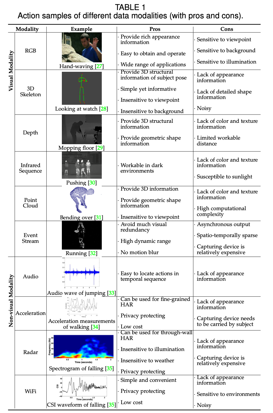A summary of data modalities in action recognition. Source: Sun et al.

Broadcast tennis matches consist of only monocular RGB video so we consider action recognition using RGB video for now.

RGB/grayscale Action Recognition

RGB video refers to video (sequences of RGB frames) captured via RGB cameras which aim to capture the colour information that a person would see. Cameras that capture in grayscale too exist, but are increasingly rare and grayscale video can often be obtained from RGB video by the colourspace conversion:

Note that other colour spaces exist, such as Hue Saturation Value (HSV) among others. These colour spaces are merely different ways of describing the colours in a frame and some are more suited to some tasks than others. HSV, for example, is preferred for colour based image segmentation.

Pre-deep learning

Before the explosion of deep learning in computer vision, handcrafted feature-based approaches were used. The most performant of these are the spatiotemporal volume based methods which attempt to capture motion descriptors in space as well as time. Examples of these features include Histogram of Oriented Gradients (HOG) which is a classic image classification feature that was extended to the temporal dimension to make a HOG3D descriptor. The HOG3D descriptor forms a class of descriptor that focuses on providing a spatiotemporal ‘view’ of an action, along with Cuboids and Spatiotemporal Orientation Analysis. Another class of descriptors focus on capturing and encoding motion information such as Motion Boundary Histograms and Histogram of Optical Flow. These features must be extracted from a video before a model such as an SVM is trained to classify them into actions.

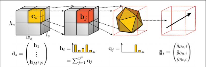An overview of the HOG3D descriptor. Source: Klaser et al.

I have experimented with extracting handcrafted features from broadcast tennis video for a classification problem, cropping around the tennis player of interest when they perform the action and using an SVM model to classify the action (a binary classification problem). I found that there was significant error as cropping around the player brought in a complex and changing background as the player was often moving, or the camera was moving (camera pan movement), or both. Background subtraction was infeasible and its’ use failed to remove features such as court lines, the net, or the line judges remaining which had a significant impact on the performance of this model. Using optical flow was problematic as, due to the view of the court from one end, the far player’s movement is often ‘suppressed’ compared to the near player and combined with the change in view from one court to another, resulting in very different looking flows for similar patterns of motion. Performance was so poor that this was not a technique that could be taken forward. On the plus side, this is also a perfect justification for using deep learning for action recognition.

An example where handcrafted features were used in combination with an SVM for tennis swing classification can be found here where the authors use Histogram of Optical Flow between frames and take a majority vote for a sequence of these features that make up an action in classifying left and right swings, achieving impressive results.

Classifiers trained on handcrafted features have achieved impressive results in the past. However, the main drawback of such models is that their ability to generalise is limited by the features extracted and since the features extracted are designed by humans, they can often be a limiting factor.

The deep learning era

Deep learning models, a fancy word for large and many-layered artificial neural networks, have seen significant success in computer vision. In the field of action recognition, deep learning has enabled us to forgo the extraction of handcrafted features and provide raw frames to models directly whereby the model learns to extract features it needs. This is facilitated by several convolutional layers which extract increasingly higher level features through the network. The ability for a model to independently learn which features are useful and how to extract them is extremely powerful and in image classification, deep neural networks have been shown to outperform other state of the art methods and we so we hope that deep learning can provide a tool to solve our problem of action recognition. However, among several drawbacks of deep learning, two are that deep models typically require a lot of data and that they are black-boxes – it can be difficult to fully understand how and why a model made a decision. In computer vision, some techniques to help understand the model more typically come in the form of visualising filters (which becomes more difficult with 3D convolutional filters) and dimensionality reduction techniques such as t-SNE or UMAP.

We can categorise the different kinds of models applied used for action recognition into one of three:

1. 2D convolutional networks
2. 2D convolutional + RNN networks
3. 3D convolutional networks

Bear in mind that this is a very broad categorisation and in practice, models can use architectural aspects of other categories. We will run through each of these designs in order.

2D convolutional networks

2D CNNs are some of the earliest models that successfully tackled the problem of action recognition. Simonyan et al. and Karpathy et al. both introduced the idea of two-stream convolutional neural networks in 2014, that used 2D convolution in both streams to classify actions, albeit in different ways.

Simonyan et al.

Simonyan et al. design a network that considers both a static RGB image in one stream to provide spatial information on what action is happening, as well as another stream that considers pre-calculated motion features.

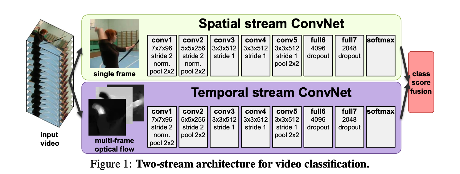Simonyan et al. two stream architecture. Source: Simonyan et al.

This paper argues that the upper stream that takes in a single RGB (3 channel) frame of spatial resolution \(w \times h\) alone is sufficient to describe the context of the activity occurring and that all that is necessary for the lower stream is a description of motion for which the authors calculate motion descriptors for \(L\) consecutive frames, where the descriptor between each frame consists of two channels describing motion in the \(x\) and \(y\) directions: \(d_t = \{d_t^x, d_t^y\}\) where \(d_t\) is the descriptor between the raw frames at time \(t\) and \(t+1\). This means \(2L\) frames are produced overall, which are stacked and passed to the lower stream which has the same spatial resolution as the static image stream of \(w \times h\) but now takes \(2L\) channels.

The authors experiment with different types of motion descriptor, experimenting with dense optical flow, trajectories and different schemas for applying these to include unidirectional flow (ie. flow in the temporal order of the frames) and bidirectional flow (consisting of computing \(L/2\) forward flows from a time \(t\) and \(L/2\) backward flows). The outputs of each stream of this network are fused using late fusion where class scores are averaged or an SVM is trained to further classify based on stream outputs.

Karpathy et al.

Karpathy et al. too designed a two-stream network, but propose using a fovea stream and a context stream.

The fovea stream takes multiple frames where each input frame is a centre crop of the original frame and the context stream takes in multiple frames that are not cropped but downsampled to a lower spatial resolution. The intuition behind this is to reduce the spatial resolution while also making use of the fact that the interesting action is generally centred in the frame for the fovea while also including wider frame context at a lower resolution.

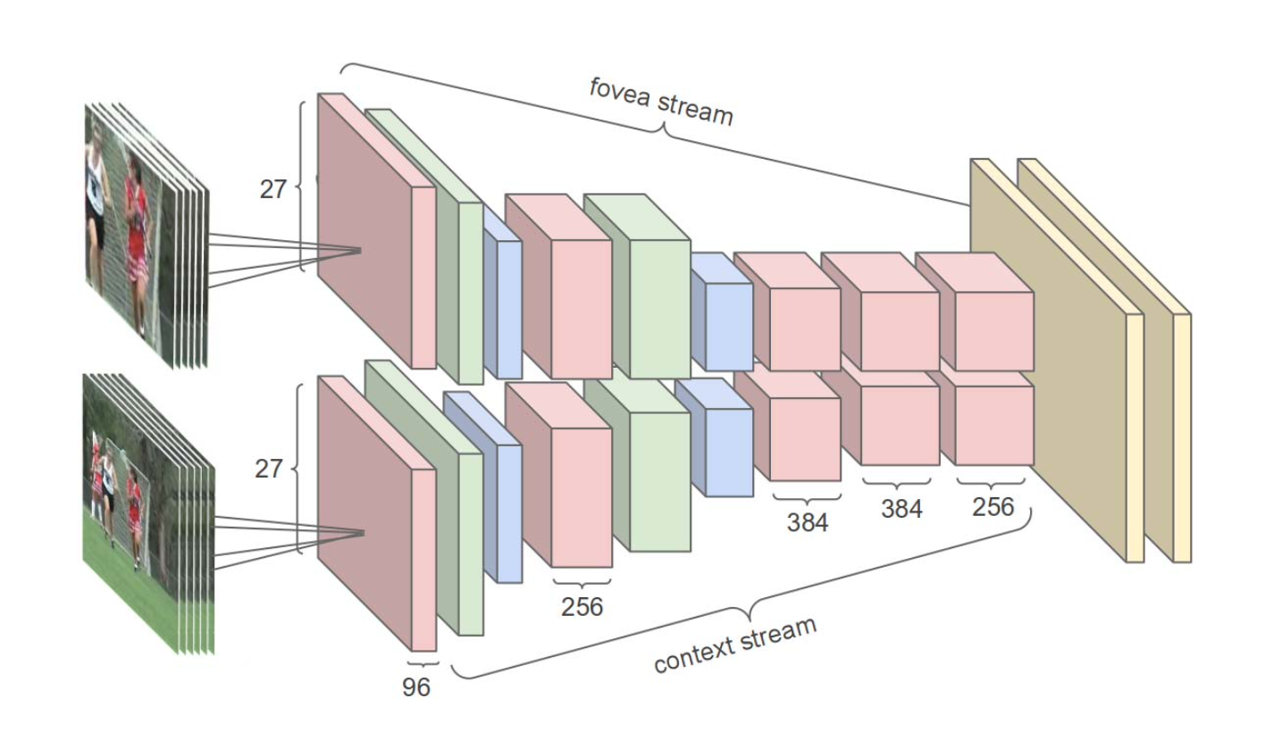Karpathy et al. two stream architecture. Source: Karpathy et al.

Perhaps most importantly, Karpathy et al. explore various methods of performing 2D convolutions on multiple frames – an idea they call Time Information Fusion – which aims to preserve temporal relationships between frames without explicitly performing temporal convolutions or use RNNs.

Karpathy et al., together with Simonyan et al., form the basis of a whole class of action recognition architectures that use 2D convolution and two streams. There are too many such models to list here, but we will go on to see just a few of the ones I think are most significant.

Feichtenhofer et al. (2016)

The previous two models, despite being two-stream models, have been separable. Each stream makes a prediction which is typically combined using an averaging mechanism or a linear model. In their 2016 paper, Feichtenhofer et al. explore different fusion techniques to better combine the spatial and temporal streams of a two-stream network.

Feichtenhofer et al. (2016) consider two kinds of fusion:

1. Spatial fusion – to better relate the spatial information from the spatial stream to the motion information in the temporal stream.
2. Temporal fusion – to combine the outputs of both the streams, which may have spatial fusion already applied

The authors use a base architecture similar to Simonyan et al., with \(L=10\) horizontal and vertical optical flow frames (making a total of \(2L\) frames) fed into the temporal stream and a standard RGB frame fed into the spatial stream. Each layer generates its own prediction which is then softmaxed and averaged to generate a combined prediction. Each stream is based on a ResNet architecture, pretrained on ImageNet.

Spatial fusion

The aim of spatial fusion is, to paraphrase the authors, to combine feature maps from the two streams at particular convolutional layers such that the channel responses of the two feature maps can interact in a (hopefully) informative way. The spatial size of two channels is easily matched, but since each layer can also have different numbers of channels, the question of how channels are allowed to interact must be answered.

Spatial fusion occurs by combing feature maps with the same spatial dimension via one of several types of interaction to include: sum fusion, max fusion, concatenation fusion, conv fusion and bilinear fusion.

The authors also consider where to fuse the networks; they consider an early fusion schema following which there is a single network to perform further convolution, as well as multiple fusion points where fusion occurs but both networks maintain their distinct streams.

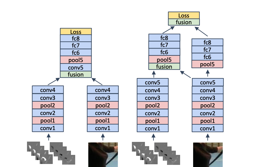Where to spatially fuse two stream architectures. Source: Feichtenhofer et al. (2016)

Temporal fusion

The standard two-stream network is fed information in a time period of \(t\pm\frac{L}{2}\) (which has total length \(L\)). However, many actions may in fact only make sense over a longer period of time. Of course, we may capture a larger frame window by, for example, considering every second frame. This, however, may well affect the computation of optical flow by violating the small motion assumption. An alternative is to consider un-strided frames over a time \(t+T\tau\) from which windows of length \(L\) are extracted and fed to the network. The feature maps generated by the inference of each window must then be fused temporally to generate a final prediction.

The authors propose two methods of temporal fusion:

1. 3D max-pooling – this is an extension of 2D max pooling
2. 3D conv + 3D max-pooling – this applies a 3D conv layer before the pooling

The authors go on to perform very in-depth experiments of the fusion strategies they propose. These results are better viewed directly in paper, if at least to save having the define and explain a range of variations of architectures.

Feichtenhofer et al. (2017)

In 2017, Feichtenhofer et al. came out with another key paper, one that explored how to share information between the two streams without explicit fusion.

The authors propose cross-stream connections – imagine residual connections as in ResNet blocks, but between streams – to allow motion information to interact directly with spatial information. They consider two ways of facilitating interactions through addition and through multiplication (Hadamard product), as well as the direction of interaction to include unidirectional interaction from the temporal to the spatial stream and vice versa, as well as bidirectional interaction. They experiment with five variations of interaction

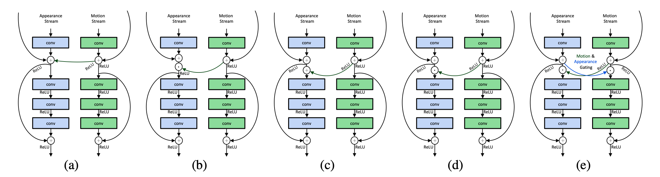Interaction variations. Source: Feichtenhofer et al. (2017)

The authors also propose a means to learn more powerful temporal features with the use of 1D convolutions in the temporal domain (rather than RNNs). The paper proceeds to experiment with various combinations of the proposed parameters and finds that unidirectional connections from the motion stream to the spatial stream using multiplication yields a significant reduction in error.

Wang et al.

In 2016, Wang et al. attempted to solve the problem of long-range dependencies; most action recognition models tend to focus on short term motion and do not provide a framework to capture long term dependencies of actions that occur over a long period of time. The authors use a two-stream approach following Simonyan et al. but develop a method to classify actions over a period longer than one clip. They call their model a Temporal Segment Network (TSN) where one input video is divided into several short sections from which a snippet of frames is selected and passed through a two-stream ConvNet. Predictions for several of these snippets are then fused to generate an overall prediction for one final prediction.

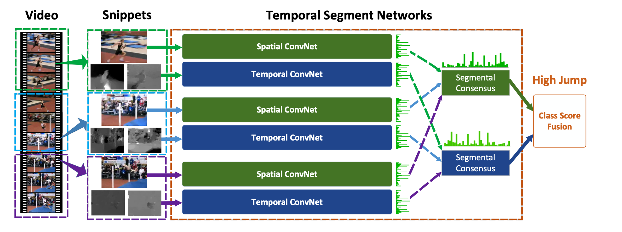Temporal Segment Network. Source: Wang et al.

The authors achieved (at the time) state of the art performance on UCF101 and HMDB51 and their approach is interesting for recognising there is a need to model long term dependencies and for providing an approach to do so.

2D convolutional network + RNN

The second class of architecture we consider are a combination of standard CNNs that employ a 2D convolutional architecture, followed by one or more RNN layers.

Early work in developing this class of model goes back to 2015, where papers by Ng et al. and Donahue et al..

Ng et al. consider raw frames (or optical flow frames) which are passed through GoogLeNet, generating a 4096 dimension feature vector for each frame. Feature vectors corresponding to each frame in a video are then either pooled or passed through an LSTM before a Softmax classifier is applied to generate a prediction. The researchers show that using LSTMs to model temporal information yields more performance than (convolutional) pooling.

Donahue et al. develop the classic CNN+LSTM model consisting of a standard 2D CNN whose features are fed into an LSTM. Several frames are fed into a model and the final prediction of the LSTM is considered the overall prediction of the model.

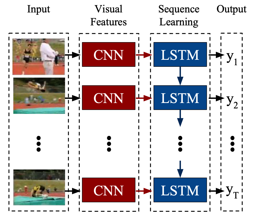CNN+LSTM model. Source: Donahue et al.

Donahue et al. consider several sub-tasks of activity recognition, image captioning and video description. For action recognition, they use an AlexNet-variant CNN along with a single layer LSTM and consider both RGB frames as well as optical flow frames as inputs. The CNN+LSTM architecture shows significant improvement over a standard single frame architecture, with optical flow-fed models outperforming RGB-fed networks. For the image captioning task, Donahue et al. also consider a two-layer LSTM and find little to no improvement in performance, concluding that additional LSTM layers do not benefit the image captioning task.

In 2016, Sharma et al. developed an extension to the standard CNN+LSTM model with the intuition that, when assessing a scene, humans focus on certain aspects of a scene at a time. This suggests that an attention mechanism may provide some benefit and so they introduce a soft attention mechanism into the model. At each time step, the CNN generates \(D\) feature map of dimension \(K \times K\) which are extracted as \(K^2\) \(D\)-dimensional vectors, each of which is passed to the LSTM layers. Each vector in the \(D\)-dimension represents different high levels features in a \(K \times K\) spatial region (this is not the input shape of the original image) and with attention, the aim is to calculate a softmax over the spatial region for each vector. Using Bahdanau Attention, the authors use the hidden state of the LSTM cell, \(\boldsymbol{h}_t\), to compute the softmax over \(K \times K\) regions at time \(t\):

Which we interpret to be the importance (distribution) over the \(K \times K\) regions. The importance is then multiplied with the feature output of the CNN, \(\boldsymbol{X}_t\) to produce the attention weighted output \(\boldsymbol{x}_t\):

\(\boldsymbol{x}_t\) is then passed on to the three-layer LSTM network.

In the realm of action recognition in tennis, this style of model has been most prevalent. I first saw this kind of model used in a 2017 paper by Mora et al. where they use Inception as the CNN followed by a three-layer LSTM. The authors use the THETIS dataset which contains labelled videos of people performing twelve tennis shots, albeit in a non-court environment. Vinyes et al. achieve impressive results across the classes, especially considering the similarity of some of the strokes (such as slice and topspin serves).

Cai et al. build on this approach, using a variation of the standard LSTM (they call this variation a historical LSTM) that adds one state, the historical state \(l_t\) at time \(t\), which is formulated based on relative values of the loss at hidden state, \(\epsilon_{h_t}\) and the loss at the historical state \(\epsilon_{l_{t-1}}\). If \(\epsilon_{h_t} > \epsilon_{l_{t-1}}\), then \(l_t\) is a combination of the previous historical state \(l_{t-1}\) and the current hidden state, \(h_t\), weighted by a learnt parameter \(\alpha_t\). Otherwise, if \(\epsilon_{h_t} < \epsilon_{l_{t-1}}\), then \(l_t\), then \(l_t\) is a weighted average of all past hidden states. In the latter case, a parameter, \(\tau\), controls the weight applied to the samples such that small \(\tau\) places an emphasis on more recent samples and vice-versa for large \(\tau\). The authors evaluate their historical LSTM with different values of \(\tau\), along with a standard LSTM and show the historical LSTM outperforming the standard LSTM. Performance is higher for smaller values of \(\tau\) suggesting that initialising \(l_t\) using more recent hidden states to update the historical state is beneficial(?).

Buddhiraju et al. perform classification on the same dataset using: 1. a variation of the CNN+LSTM model that replaced the LSTM with a bidirectional LSTM; and 2. an architecture found via architecture search using EvaNet, achieving near identical performance with both models on a reduced, six class problem.

Faulkner et al. perform work similar to Donahue et al. with a tennis-specific focus, attempting to recognise and events in tennis and then segment them, as well as generate commentary on the event. They evaluate several different architectures such as a CNN+LSTM model, full 3D conv models as well as two-stream architectures and find, for segmentation that two-stream models and CNN+LSTM models perform better. Their work only touches on action classification, preferring to detect serves or hits in one of four regions on screen, but is an interesting read.

3D convolutional networks

3D ConvNets see their origin in a 2012 paper called 3D Convolutional Neural Networks for Human Action Recognition. 3D convolution is a straightforward extension of standard 2D convolution. In 2D convolution, the value at a position \(x, y\) in the \(j\)-th feature map in the \(i\)-th layer is given by \(v^{x, y}_{i, j}\):

where \(P_i, Q_i\) are the convolution kernel height and width, respectively, and after which a bias and/or activation can be applied. 2D conv is just a weighted sum of a particular value and its immediate neighbours in the x-y plane. 3D conv takes this a step further adding another dimension in the z-plane. So, a value at the location \(x, y, z\) is now given by:

With a convolution kernel of dimension \(R_i\) in the z-dimension.

The idea of 3D convolution is key as it allows direct learning of features from the time(z) dimension vie convolution which enforces locality and, with deeper layers, allows longer-range interactions. This idea has spawned many architectures such as C3D, I3D (which directly expands a 2D CNN, two-stream architecture into a two-stream 3D architecture) as well as more recent architectures such as (very interesting) SlowFast and X3D. 3D convolution architectures, unlike their CNN-LSTM counterparts, take as input a clip made of a fixed number of frames e.g. a 16 frame clip consists of 16 frames in order and convolution is performed directly on these.

The obvious disadvantage of 3D convolution compared to 2D convolution is the increase in parameters – the weight tensors go from being ‘flat’ and two-dimensional to 3D weight cubes. This increases parameters and training hardware requirements (as more gradients etc. must be stored) is easier to overfit. Some approaches to enable convolution in the temporal dimension while also minimising the number propose separating the spatial and temporal convolutions with the idea that separable spatial and temporal convolution can approximate a full, single unified convolution. R(2+1)D is one design that extends ResNet, adding explicit temporal-only convolutions to each block.

Just for fun: 4D convolution

In 2020, Zhang et al. published a paper that aims to overcome the limitations of 3D ConvNets – namely the limitation in the number of frames in a clip. The clip size is typically small, perhaps 16-32 frames, but, in the real world many videos can be much longer with Kinetics-400 videos typically 36-72 frames long. The authors of this paper propose splitting up a whole video into action units, \(A_i\), which are short clips that represent a portion of an action. Multiple action units extracted in-order from a video make up a video input \(V = {A_1, ..., A_U}\) where \(A_i \in C \times T \times H \times W\) for \(U\) action units in a video. The authors intuit that rather than using longer clips with 3D convolution, where finding long-term (temporal) relationships would require deeper networks, using 4D convolutions across clips would better model long-term interactions.

Mathematically, 4D convolution is a straightforward extension of 3D convolution that adds another dimension of parameters to a weight matrix and requires one more sum over the fourth dimension.

Zhang et al. implement 4D convolution using an I3D ResNet-18 base and add a 4D residual block. This is likely better understood with the figure below from their paper.

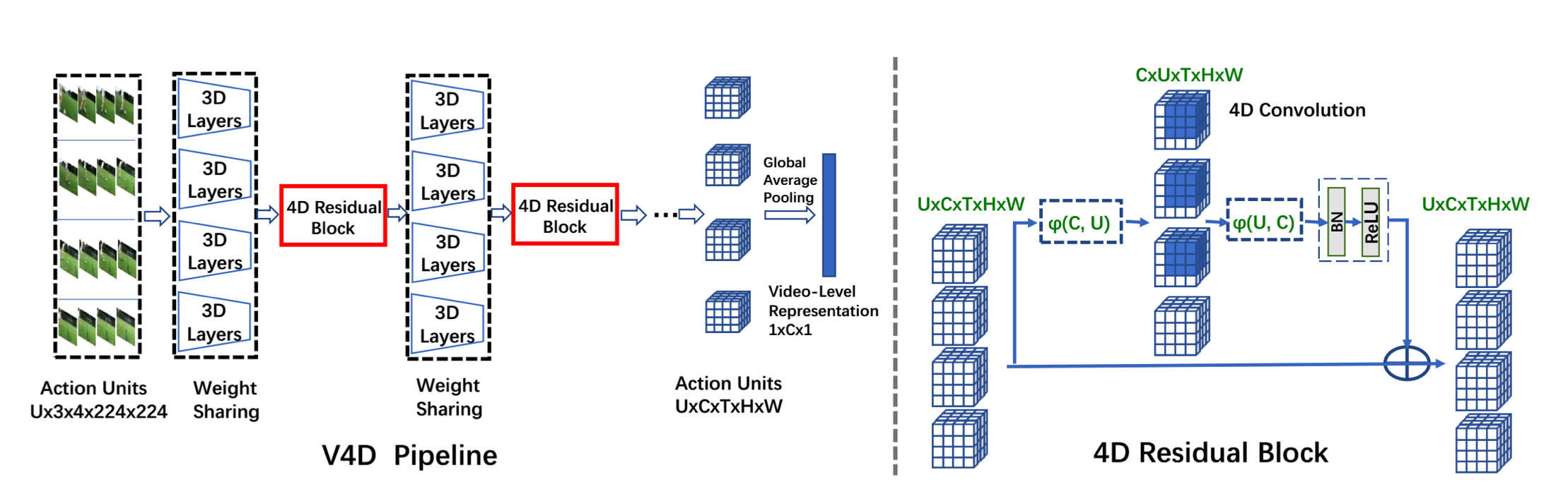Interaction variations. Source: V4D design, Zhang et al.

Using 4D convolutions begs one question: if the aim is to model long term dependencies, then why not use a 3D CNN+LSTM combination? It at least makes an interesting comparison to convolution across clips. I haven’t yet come across a paper that does experiments with this combination on a dataset like Kinetics, although You et al. use this setup for a Video Quality Assessment task.

Summary

We have run through some of the important papers in action recognition and have covered a variety of approaches to solving problems in this area. This is hardly an exhaustive list and a quick search for summaries yields papers that list key literature in chronological order.

We have more or less stuck to exploring RGB video derivative modalities, but, there are other types of data that are available depending on the application. Another key part of action recognition is data; datasets have been getting bigger over the years and modern architecture evaluation is often performed with multiple datasets. Understanding the data is as important as understanding the model itself.

Human action recognition is an active research area and new approaches consist of new designs, new ways of manipulating data as well as new components to eke yet more performance out of existing models. Some of the challenges in this field are background clutter, fast motion, occlusion, viewpoint changes and changes to illumination.