This post, and indeed the successive posts in this series are focused on portfolio optimisation. Harry Markowitz is credited with developing the field of Modern Portfolio Theory, and won the Nobel Prize in Economics for developing the Markowitz Model (Minimum-Variance).
Understanding Return and Risk
When we look at an investment opportunity, we are concerned only with the Return offered by the venture and the risk associated with it. Return or Return on Investment (ROI) is a measure of how much as a percentage we expect to earn from an initial investment.
\[\begin{align} ROI = \frac{\text{final value of investment} - \text{initial value of investment}}{\text{cost of investment}} \times 100\% \end{align}\]When looking at a series of returns, such as daily stock returns over the past k days we may see something like this:
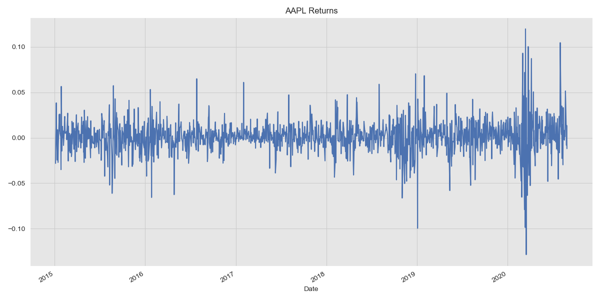 AAPL daily returns
We expect returns to be normally distributed with some mean \(\mu\) and standard deviation \(\sigma\).
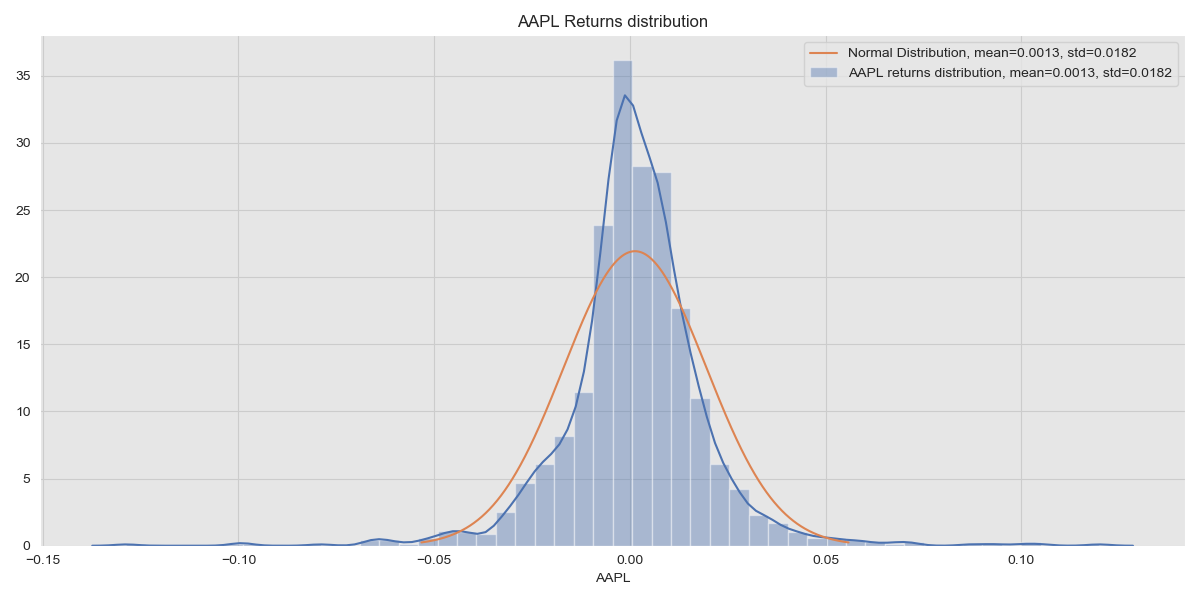 AAPL returns distribution
The returns distribution is a little different to the Normal distribution plotted and this is because we don’t consider the higher moments.
AAPL’s returns here show a mean (expected) daily return of 0.13% and a standard deviation of 1.8%. The standard deviation of a distribution represents the spread of the values around the mean and as a result, this is a direct measure of the volatility of the returns of a security. Generally, an increase in volatility corresponds to an increase in risk and Markowitz argues that volatility can be taken as a proxy for risk and so standard deviation can be used instead of risk in calculations.
When presented with a world of stocks, such as some of the constituents of the S&P 500, we turn to linear algebra to keep notation concise. For a single stock the mean return, \(\mu\) is a scalar value and when extended to multiple stocks corresponds to a vector:
\[\begin{align} \mu = \begin{bmatrix} \mu_1 \\ \mu_2 \\ ... \\ \mu_n \end{bmatrix} \end{align}\]We also define the covariance matrix, \(\Sigma\), which is a measure of the linear relationship of the returns between two assets.
\[\begin{align} \Sigma = \left[ \begin{array}{ccc} \sigma_{11} & \cdots & \sigma_{1n} \\ \vdots & \ddots & \vdots \\ \sigma_{n1} & \cdots & \sigma_{nn} \end{array} \right] \end{align}\]An important note!
When discussing returns in this post, we assume linear returns only. Log-returns are another method for calculating returns and the Portfolio Theory used here will not work for log-returns without modification.
Investment Objectives
When making an investment, intuitively, we want to choose investments that minimise risk (perhaps while also achieving a certain level of return). When choosing which stocks to invest in from a world of stocks, if we being with initial capital c, we want to find the best possible way of allocating portions of this money to buying a selection of stocks such that we satisfy our investment objectives. Rather than solving the problem of exactly how much capital to allocate to buying each stock, we instead solve the problem of what proportion of the initial capital should be allocated to each stock. We define a weight vector, \(w\), which allows this.
\[\begin{align} w = \begin{bmatrix} w_1 \\ w_2 \\ ... \\ w_n \end{bmatrix} \end{align}\]Now, to ensure that we are investing only the money we have we have to apply the constraint that the sum of the values in the weight vector is equal to 1.
\[\begin{align} \sum_{i = 1}^{n} w_i = e^Tw= w^Te = 1 \end{align}\]Where \(e\) is a vector of ones.
Given the covariance matrix, we can calculate the variance of a portfolio defined by weights \(w\) using:
\[\begin{align} variance = w^T \Sigma w \end{align}\]Similarly, we can also calculate the expected returns of a portfolio as:
\[\begin{align} return = w^T \mu = \mu^T w \end{align}\]Now that we have found a way of defining portions of our objective mathematically, we can solve our investment problem mathematically. As stated before, we want to minimise the risk associated with our portfolio while at the same time achieving a particular level of return.
We can start this off as a minimisation problem and add constraints that demand a level of return and place limits on the available capital.
\[\begin{align} \underset{w}{\mathrm{argmin}}\ w^T \Sigma w\\ \mathrm{subject\ to} \\ w^T \mu = r \\ w^T e = 1 \end{align}\]We choose to solve this problem as it can be done parametrically. We rewrite the problem slightly as follows:
\[\begin{align} \underset{w}{\mathrm{argmin}}\ \frac{1}{2}w^T \Sigma w\\ \mathrm{subject\ to} \\ w^T \mu - r = 0 \\ w^T e - 1 = 0 \end{align}\]Note that we introduce a factor of \(\frac{1}{2}\) into the minimisation problem as this cancels out a multiplier constant (as we will see) as well as move all the values to one side of the equation in the constraints. We are now ready to solve this problem. This portfolio also allows short selling of stocks as we place no requirement that each weight is positive, merely that the sum of the weights is 1.
Solving different optimisation problems
There are many different ways of solving the problem to find an optimal portfolio. For example, we could choose that we are not interested in achieving excess (above market) returns at all and that we are extremely risk averse. In this case we could rewrite the optimisation problem as:
\[\begin{align} \underset{w}{\mathrm{argmin}}\ \frac{1}{2}w^T \Sigma w\\ \mathrm{subject\ to} \\ w^T e - 1 = 0 \end{align}\]If we refuse to short sell stocks than we can introduce another constraint:
\[\begin{align} w_i \geq 0\ \forall i \in \{1, 2, \dots, n\} \end{align}\]We can also solve an optimisation problem to find the maximum possible return while also minimising the variance:
\[\begin{align} \underset{w}{\mathrm{argmin}}\ \frac{1}{2}w^T \Sigma w - q w^T \mu\\ \mathrm{subject\ to} \\ w^T \mu - r = 0 \\ w^T e - 1 = 0 \end{align}\]Where \(q \in [0, \infty)\) is a ‘risk tolerance’ factor. Some of these problems can’t be solved parametrically and require Quadratic Programming packages to solve.
Back to our problem
We now return to our problem.
\[\begin{align} \underset{w}{\mathrm{argmin}}\ \frac{1}{2}w^T \Sigma w\\ \mathrm{subject\ to} \\ w^T \mu - r = 0 \\ w^T e - 1 = 0 \end{align}\]We proceed to solve this problem using Lagrange Multipliers, writing the Lagrangian as follows.
\[\begin{align} L(w, \alpha, \beta) = \frac{1}{2}w^T \Sigma w - \alpha (w^T \mu - r) - \beta (w^T e -1) \end{align}\]We differentiate to obtain the optimality conditions.
\[\begin{align} \frac{dL}{dw} = \Sigma w - \alpha \mu - \beta e = 0 \\ \frac{dL}{d \alpha} = w^T \mu - r = \mu^T w - r = 0 \\ \frac{dL}{d \beta} = e^T w - 1 = 0 \end{align}\]We can rewrite the optimality conditions in one equation.
\[\begin{align} \begin{bmatrix} \Sigma & -\mu & -e \\ -\mu^T & 0 & 0 \\ -e^T & 0 & 0 \end{bmatrix} \begin{bmatrix} w \\ \alpha \\ \beta \end{bmatrix} = \begin{bmatrix} \mathbf{0} \\ -r \\ -1 \end{bmatrix} \end{align}\]Which we can solve by:
\[\begin{align} \begin{bmatrix} w \\ \alpha \\ \beta \end{bmatrix} = \begin{bmatrix} \Sigma & -\mu & -e \\ -\mu^T & 0 & 0 \\ -e^T & 0 & 0 \end{bmatrix}^{-1} \begin{bmatrix} \mathbf{0} \\ -r \\ -1 \end{bmatrix} \end{align}\]Now that we have the method to find the solution, we can start writing some code!
Finding the Optimal Portfolio
As we have seen, we need to look at returns for a number of stocks and from these, calculate a mean vector and covariance matrix. We begin by importing the necessary packages and getting the adjusted closing prices.
1
2
3
4
5
6
7
8
9
10
11
12
13
 import numpy as np
 import pandas as pd
 import matplotlib.pyplot as plt
 import pandas_datareader.data as pdr
 import datetime as dt
 import seaborn as sns
 from scipy import stats

 start = datetime.datetime(2015, 1, 1)
 end = datetime.date.today()

 data = pdr.DataReader(nasdaq_100_tickers, "yahoo", start, end)
 data = data["Adj Close"]
From this we calculate daily returns for each stock and split the dataset, taking the final 252 days as an Out Of Sample (OoS) test set. We make sure to calculate returns over a period of 252 days, as there are 252 (ish) working days in a year. This also lets us demand a set annual return (let’s just say we generate returns only on working days) rather than have to compute which average daily return corresponds to a required annual return.
1
2
3
4
5
 returns = data.pct_change().dropna()
 test_set = returns[-252*4:]
 train_set = returns[:-252*4]
 mu = train_set.mean().values.reshape(-1, 1)
 sigma = train_set.cov().values
Next, we construct the augmented matrices that we need to solve our problem.
1
2
3
4
5
6
7
8
9
10
 r = 0.25 # Required return
 num_stocks = returns.shape[1]
 e = np.ones(num_stocks).reshape(-1, 1)
 zero = np.zeros(num_stocks).reshape(-1, 1)
 one = [[1]]
 zero = [[0]]
 zero_vec = np.zeros(num_stocks).reshape(-1, 1)

 augL = np.vstack( ( np.hstack((sigma, -mu, e)), np.hstack((-mu.T, zero, zero)), np.hstack((-e.T, zero, zero)) ) )
 augR = np.vstack( (zero_vec, -r, one) )
We can now find the solution to this problem.
1
2
3
4
5
 result = np.dot(np.linalg.inv(augL), augR)

 w = result[:-2]
 alpha = result[-2]
 beta = result[-1]
We can verify that we are not spending more money then we have by computing the sum of \(w_i\)’s.
1
 w.sum() == 1.0
This yields one, confirming that we are not spending money we don’t have.
To see how this portfolio performs, we can calculate the returns on both the In Sample (train) data and the OOS (test) data.
1
2
3
4
5
6
7
8
9
10
11
12
13
14
15
16
17
18
19
20
21
22
23
24
25
26
27
28
29
30
31
32
 eq_w = np.ones(num_stocks) / num_stocks # Ratios for an equally weighted portfolio

 train_cust_ret = []
 test_cust_ret = []
 test_eq_ret = []
 train_eq_ret = []

 for row in train_set.values:
 train_cust_ret.append(np.sum(np.dot(w.T, row)))
 train_eq_ret.append(np.mean(row))

 for row in test_set.values:
 test_cust_ret.append(np.sum(np.dot(w.T, row)))
 test_eq_ret.append(np.mean(row))

 train_cust_ret = np.array(train_cust_ret)
 test_cust_ret = np.array(test_cust_ret)
 test_eq_ret = np.array(test_eq_ret)
 train_eq_ret = np.array(train_eq_ret)

 x = np.linspace(1, len(train_set)+len(test_set), len(train_set)+len(test_set))

 plt.plot(x[:len(train_set)], np.cumprod(1+train_cust_ret), label="Custom Portfolio, In Sample")
 plt.plot(x[len(train_set):], np.cumprod(1+test_cust_ret), label="Custom Portfolio, Out Of Sample")
 plt.plot(x[len(train_set):], np.cumprod(1+test_eq_ret), label="Equally weighted portfolio returns, In Sample")
 plt.plot(x[:len(train_set)], np.cumprod(1+train_eq_ret), label="Equally weighted portfolio returns, Out Of Sample")
 plt.legend()
 plt.title("Portfolio returns vs Equally Weighted Portfolio Returns")
 plt.xlabel("Days since beginning")
 plt.ylabel("Return")
 plt.tight_layout()
 plt.show()
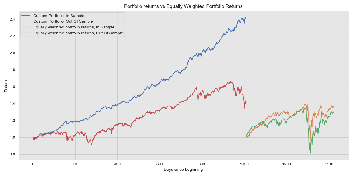 Portfolio Performance on In Sample and Out Of Sample data
As we expect, the In Sample performance is brilliant (this is akin to testing performance on training data), whereas the portfolio constructed from the In Sample data performs markedly less spectacularly in OOS data. Looking at the OOS results more closely, see that the Equally Weighted Portfolio generated a return of 30.11% whereas our portfolio managed a return of 35.62%. Sure, we’re winning, but not by much!
Another way of thinking about portfolios
Till now, we have considered finding an optimal portfolio as an optimisation problem. Let’s take the problem finding the minimum variance portfolio:
\[\begin{align} \underset{w}{\mathrm{argmin}}\ w^T \Sigma w\\ \end{align}\]We attempt to minimise the covariance matrix, which is a positive (semi-)definite matrix that does have an inverse. As the covariance matrix is symmetric all its eigenvectors are mutually orthogonal. The eigenvalues representing the risk associated with each eigenvector, which itself is a vector of weights of the constituents in that portfolio. As a result, choosing to build a portfolio corresponds to the eigenvector of the smallest eigenvalue will yield the least ‘risky’ portfolio. Also, the largest eigenvalue corresponds to the portfolio most strongly correlated with the market (the market created by the data that is used) and some techniques recommend ignoring the eigenvector associated with this eigenvalue as the whole aim is to decorrelate portfolio returns from the market as much as possible.
Why does this work? Well, to understand this it is best to look at stock returns as a signal.
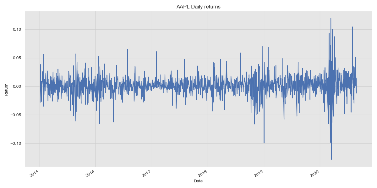 AAPL returns
This signal as a whole is made up of a bunch of other signals which when combined in some fashion yield the signal we see. We can find these sub-signals by computing the eigendecomposition which yields a bunch of eigenvalues and eigenvectors. The eigenvalues indicate how much of a particular sub-signal contributes to the overall signal and so the eigenvector corresponding to the largest eigenvalue is supposed to explain the most (relatively) variance out of all the sub-signals. As we consider more sub-signals in order of decreasing eigenvalue, we get closer to constructing the original signal. For an excellent intuitive explanation of this, read this.
With that out of the way, we can explore how to find some portfolios using an eigendecomposition method. We begin with the returns previously computed and calculate the mean and covariance matrices.
1
2
3
4
5
 returns = data.pct_change().dropna()
 train_set = returns[:252*4]
 test_set = returns[252*4:]
 mu = train_set.mean().values.reshape(-1, 1)
 sigma = train_set.cov().values
Computing the eigendecomposition yields the eigenvectors and eigenvalues.
1
2
 eigvals, eigvecs = np.linalg.eigh()
 # Eignevalues and eigenvectors are already ordered smallest-largest
From this, we can look at the components of each stock in each portfolio, after normalising the eigenvector to one.
1
2
3
4
5
 portfolio1 = eigvecs[-1]/np.sum(eigvecs[-1]) # Portfolio correspond to largest eigenvalue
 plt.bar(returns.columns[:20], portfolio1[:20])
 plt.title("Portfolio 1")
 plt.tight_layout()
 plt.show()
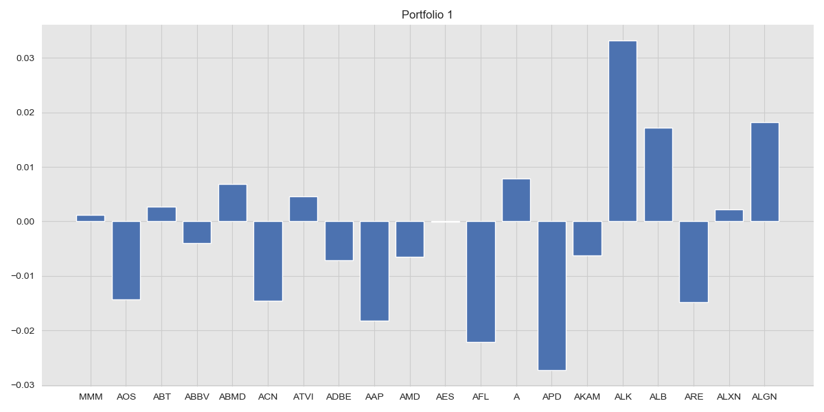 Portfolio 1
As mentioned before, we want a portfolio that is less correlated with the market and so we discard the largest eigenportfolio and instead choose the second largest. As in the previous section, we can visualise how well this portfolio performs. Note that here, we have placed no demand of a required rate of return.
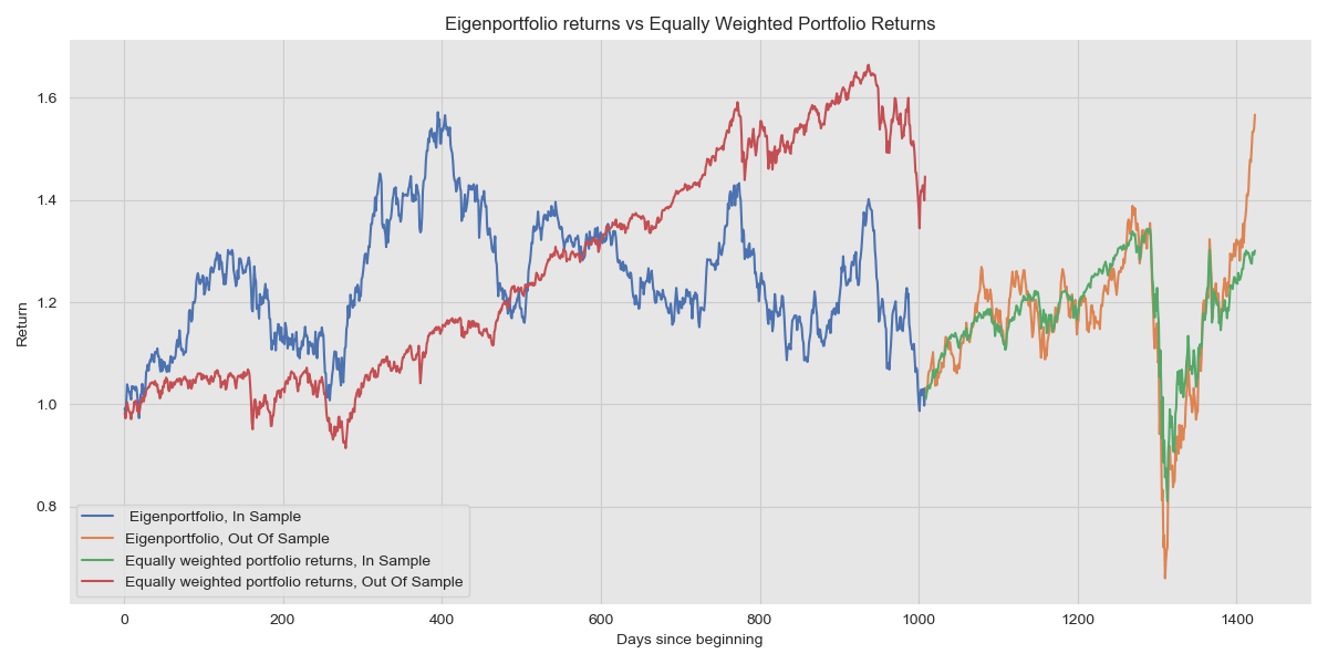 Eigenportfolio
This highlights the performance of the riskiest portfolio that isn’t the market portfolio and we can use lower variance portfolios. Using the portfolio that corresponds to the smallest eigenvalue yields:
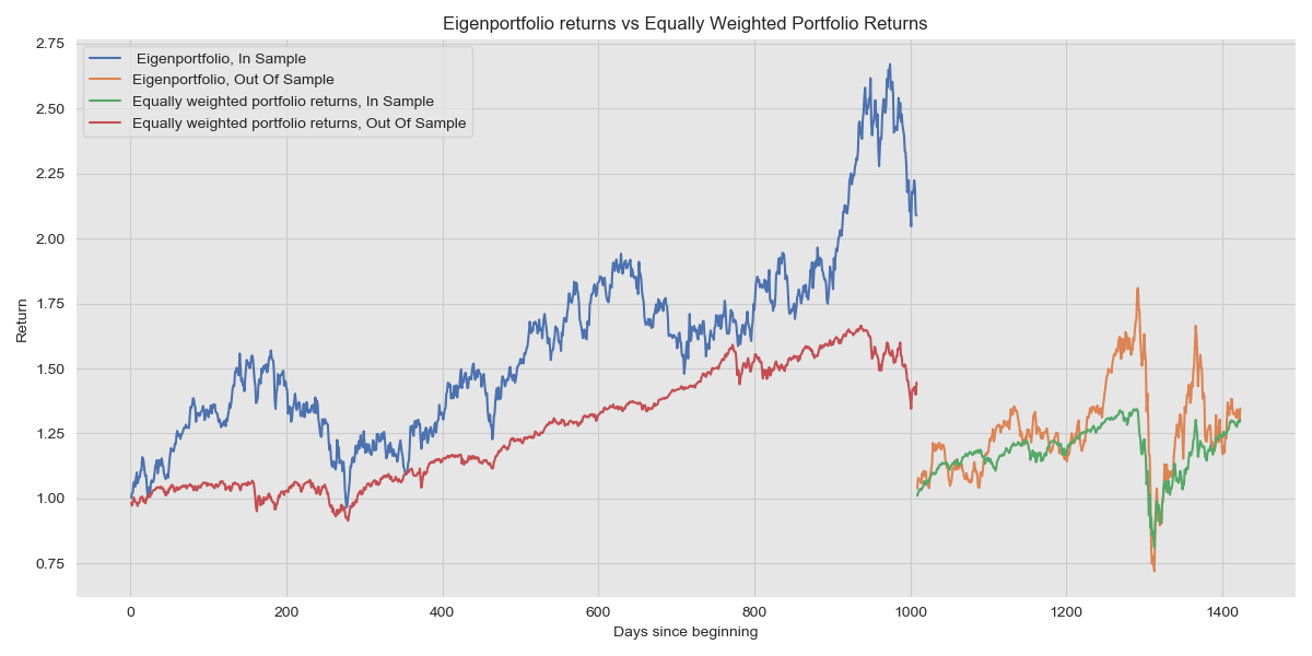 Eigenportfolio
What next?
At this point, we are only beginning to realise the potential of Modern Portfolio Theory. This introduction leaves several questions unanswered:
-
How can we try and eke more performance out of a portfolio by choosing a portfolio that is more likely to yield higher returns.
-
How can we deal with sampling error?
-
How can we ditch a bad strategy before we take too high a loss?
These are some of the questions I want to explore in future posts in this series. Given my snail’s pace posting rate it may be a while, but I will post in time. In the meantime, you may enjoy some of my other blog posts.