Another day, another post. This time it’s all about Momentum. Momentum is, as defined in the Oxford English Dictionary:

1. The ability to keep increasing or developing

2. A force that is gained by movement

3. (specialist) The quantity of movement of a moving object, measured as its mass multiplied by its speed.

Anyone who has taken a beginner/intermediate level Physics class in school is likely intimately familiar with momentum as a concept – something to do with how fast an object is going and how much it weighs. Perhaps the most important takeaway from that class is the idea that we can use momentum to decide what the aftermath of a collision is likely to look like (see Conservation of Momentum). On a more intuitive level, you may remember this: stopping a heavy, moving vehicle is difficult!

We extend this idea to equity prices; if a stock has been performing well, then it is likely to perform well in the future, and conversely, underperforming stocks are likely to underperform in the future. Jegadeesh and Titman developed the foundation for momentum-based strategies, which, contrary to the prevailing theory of mean-reversion, argued that trends persist and developed the Relative Momentum (RV) strategy. Note that Relative Momentum is also called Cross-Sectional Momentum.

The Intuition

In a nutshell, in a world with n securities, Relative Momentum works as follows every time we want to rebalance the portfolio:

1. Calculate returns for the past k months for each stock

2. Sort the stocks into then decile equally weighted portfolios.

3. At rebalance time, go long on the top-performing m portfolios and short the m worst performing portfolios, making sure to close any previous positions taken at the last rebalance time.

Straying a little from Jegadeesh and Titman’s approach, we are going to sort the stocks based on past k month returns, and not into decile equally weighted portfolios.

Obtaining Data

To obtain data, we defer to pandas-datareader using which we download data from 2015 to the present for stocks in the S&P 500, using Yahoo Finance as the data source. We follow this up by removing any tickers with missing data for these dates.

1
2
3
4
    start = dt.datetime(2015, 1, 1)
    end = dt.datetime.now()
    df = pdr.DataReader(tickers, data_source="yahoo", start=start, end=end)
    df = df.dropna(axis=1)

We can then look at some of the prices for these over time. We will use the Adjusted Close prices for the remainder of this post.

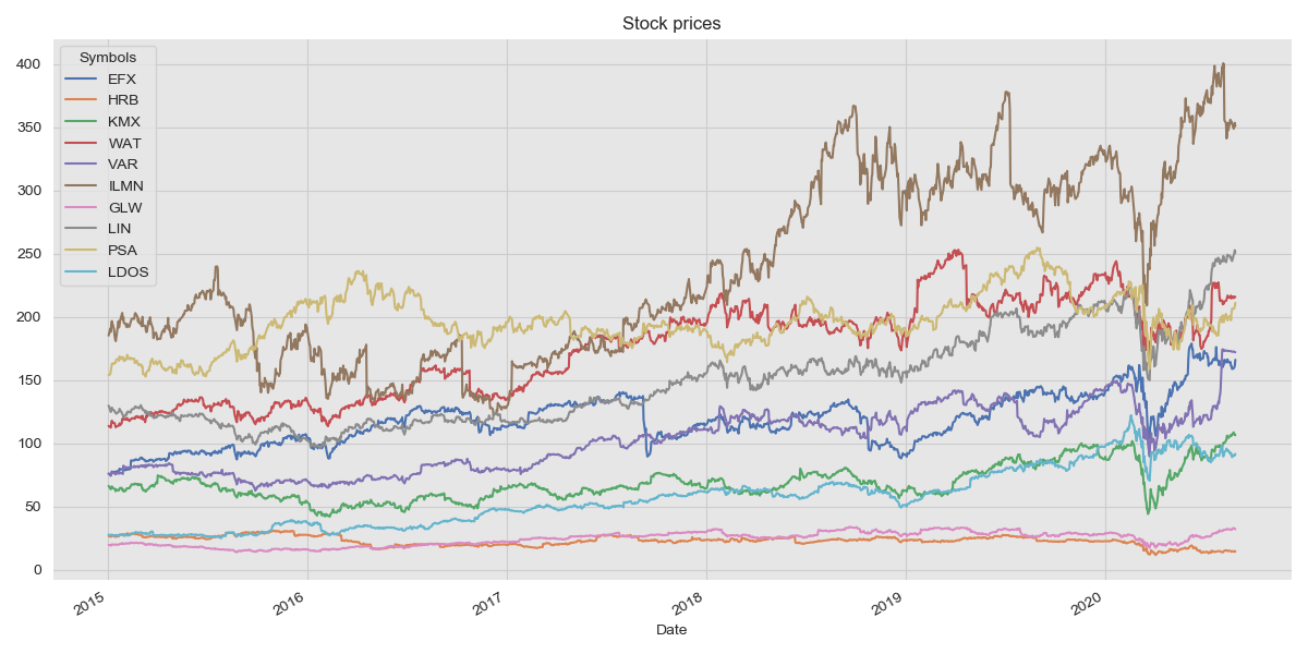Stock prices over time

Implementing Relative Momentum

The crux of the Relative Momentum trading strategy is to use returns for the last k days as the momentum. We can calculate the returns for every period as follows:

1
2
    adj_close = df["Adj Close"]
    pct_changes = adj_close.pct_change(momentum_period).dropna()

We also need to know which the rank of each stock at every stage. To do this, we initialise a new Dataframe and fill it with the ranks. We remember to shift this forward by one day because at rebalance time, we only have information up till the previous day.

1
2
3
4
5
6
7
    df_ranks = pd.DataFrame(columns=pct_changes.columns, index=pct_changes.index)
    for i in range(len(pct_changes)):
        if i % rebalance_freq == 0:
            df_ranks.iloc[i] = pct_changes.iloc[i].rank(axis=0, ascending=False)

    df_ranks = df_ranks.shift(periods=1, axis=0)
    df_ranks.ffill(inplace=True)

With the machinery in place, we can go ahead and simulate some trades!

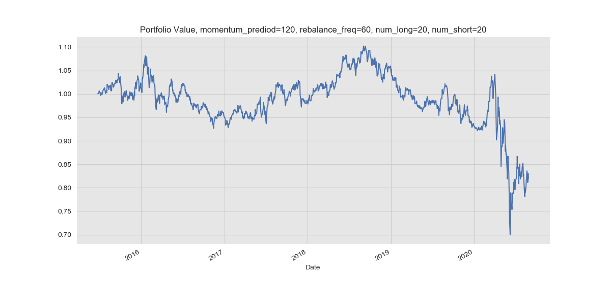
We are left to choose how many stocks we take a long position on and how many we short at each rebalance time. We begin with a balanced 20 long, 20 short.

1
2
3
4
5
6
7
8
9
10
11
12
13
    num_long = 20
    num_short = 20
    num_stocks = df_ranks.shape[1] - num_short + 1

    for col in df_ranks.columns:
    # If a stock is ranked within the top num_long, we take a long position
    df_ranks.loc[df_ranks[col] <= num_long, col] = 1

    # If a stock is ranked in the bottom num_short, we short it
    df_ranks.loc[df_ranks[col] >= num_stocks, col] = -1

    # Otherwise do nothing
    df_ranks.loc[(df_ranks[col] < num_stocks) & (df_ranks[col] > num_long), col] = None

To view how well the strategy has performed we also need to calculate how our money changes in value over time.

1
2
3
4
5
6
7
8
    res_df = (adj_close.pct_change()) * df_ranks
    res_df['Total Return'] = (res_df.sum(axis=1, skipna=True)) / (num_long + num_short)
    res_df = res_df[momentum_period:]
    res_df['Portfolio Value'] = ((mult_df['Total Return'] + 1).cumprod()) * 1

    res_df['Portfolio Value'].plot()
    plt.title(f'Portfolio Value, momentum_prediod={momentum_period}, rebalance_freq={rebalance_freq}, num_long={num_long}, num_short={num_short}')
    plt.show()

So how does our strategy perform?

Varying the strategy

This trading strategy affords us a lot of freedom to change the parameters. We can change the rebalance frequency, the momentum period or the number of stock we take long or short positions on.

So, let’s explore what happens when all we do is taking long positions.

1
2
    num_long = 20
    num_short = 0

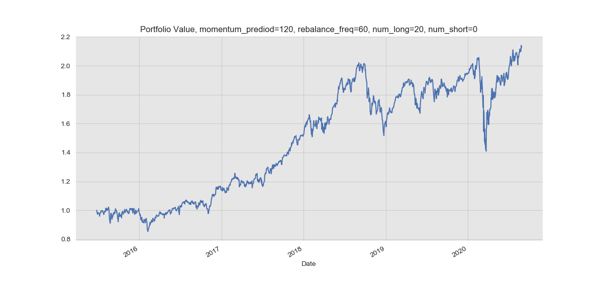
It turns out that this strategy seems successful – at least we are now making money – but the average annual return is approximately 16.4%. This is respectable, but a far cry from being a successful trading strategy. On closer inspection, we see that the strategy returns less than 4% for the first two years. This means that for this period, you would be better off investing in an index fund; the S&P 500 has averaged an annual return of 10% through till 2019. We also have to bear in mind that the real return is likely to be lower as we haven’t accounted for the cost of trading yet, and passive funds have very low Annual Management Charges.

We next turn to shorting, and see how a pure shorting strategy performs.

1
2
    num_long = 0
    num_short = 20

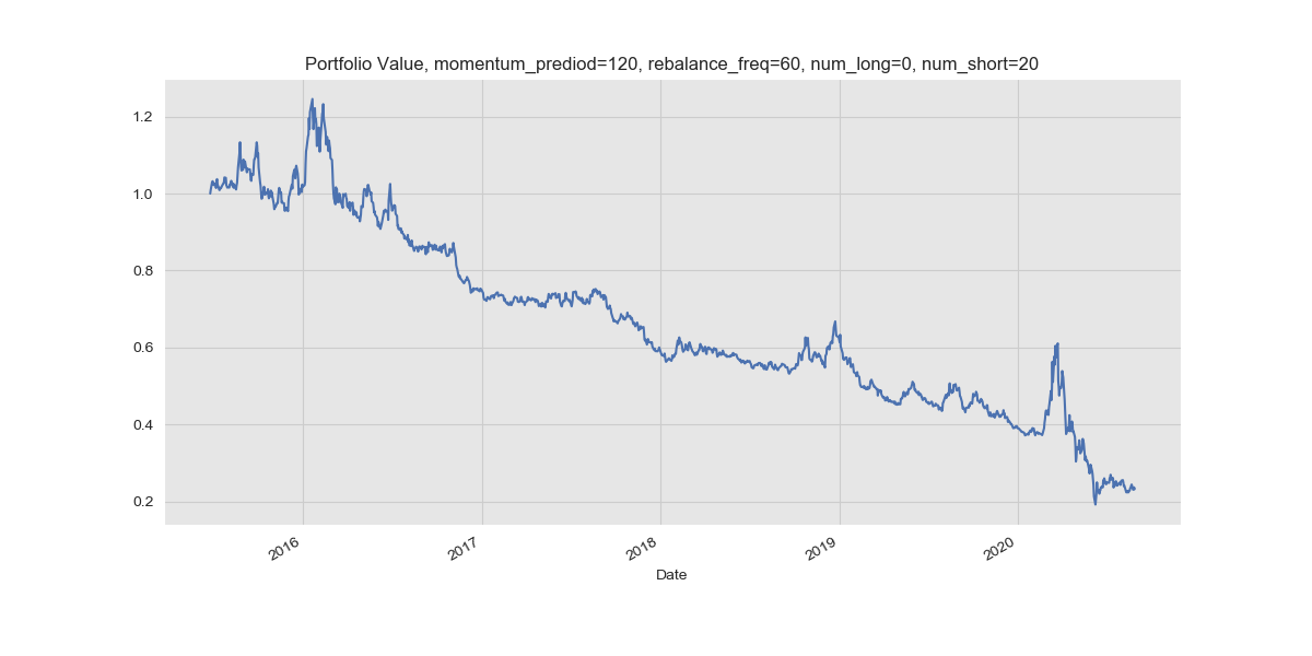
The shorting strategy performs spectacularly poorly losing nearly 80% of the portfolio value over the five years. However, shorting typically aims to exploit recent and short term drops in stock prices (see this for a description of shorting) and our use of a 120 day momentum period may be causing this strategy to backfire. We adjust the momentum period and rebalance frequency and repeat this strategy.

1
2
    momentum_period = 5
    rebalance_freq = 5

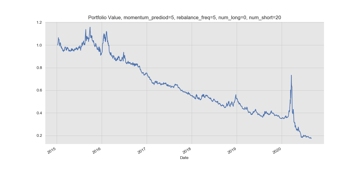
As before we see a circa 80% decline in portfolio value. The most interesting part, however, is the spike in value in early 2020. This corresponds to the market crash due to Coronavirus and highlights the use of a shorting strategy in a bear market.

Finally, we also want to see how a simple buy and hold strategy compares with Relative Momentum. We build an equally weighted portfolio of each of these stocks and see a return of 100.79%! Now, saying that Relative Momentum is useless is a blanket statement – it has its uses in a carefully analysed environment with appropriate variables but it certainly isn’t the kind of strategy you want to leave running in the long term.

Wrapping up

We have merely explored a clean, academic implementation of the Relative Momentum strategy. A true trading environment would have far more sophisticated back-testing and robust code, but this serves the purpose of exploring the strategy and understanding why it works (or doesn’t work). For an insight into what a momentum strategy looks like in a production environment, head over to one of the many algorithmic trading platforms with far more software engineer-y implementations.