After taking the course, Mathematics for Machine Learning (MML), at university and reading the excellent book of the same name, I was well and truly hooked on Gaussian Processes. The MML book introduces the idea of applying the full Bayesian treatment to Linear Regression, leading to the simple and beautiful Bayesian Linear Regression. The book, Gaussian Processes for Machine Learning (GPML), tackles Gaussian Processes in much more detail and the rest of this post leans extensively on the material covered in Chapter 2. A great way to get started with the intuition and theory behind Gaussian Processes is to read Chapter 9 of the MML book, after covering Chapters 1-7 which runs through the required mathematics.

What is a Gaussian Process? In a nutshell, any possible number of functions can explain a set of observed data and Gaussian Processes assign a probability to each of these possible functions. This results in a probability distribution which allows us to make point estimates in addition to characterising the uncertainty of a prediction.

With that out of the way, let’s get started.

Generating Data

In the real-world data can be generated by any function. This function is usually unknown and the role of machine learning is to try and find this function using observations. To make matters more complicated real-world data is often noisy. We model the function of the observations as \(y = f(x) + \epsilon\) where \(f(x)\) is the underyling function generating data in the real-world and \(\epsilon\) is a noise term, \(\epsilon \sim N(0, \sigma_n^2)\). Note that \(f(x)\) is not necessarily a linear function. We consider the data generating function \(f(x) = sin(2\pi x) + cos(9\pi x)\).

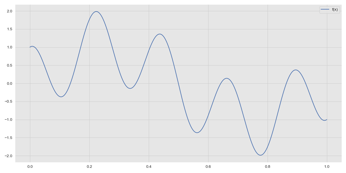Function \(f(x) = sin(2\pi x) + cos(9\pi x)\)

We obtain 1000 observations, but this is unrepresentative of real-world data; we still need to add some noise. We set the standard deviation of the noise term, \(\sigma_n = 0.4\) and sample the distribution for \(\epsilon\) 1000 times and add these to the values of \(f(x)\).

1
2
3
4
5
6
    n = 1000
    x = np.linspace(0, 1, n)
    f = lambda x: np.sin(2*np.pi*x) + np.cos(9*np.pi*x)
    sigma_n = 0.4
    epsilon = np.random.normal(loc=0, scale=sigma_n, size=n)
    y = f(x) + epsilon

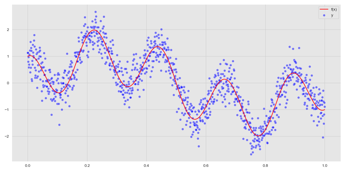\(y = f(x) + \epsilon\)

The choice of \(\sigma_n\) determines how noisy the observations are. The errors, that is, the differences between the observations and the function \(f(x)\) should be normally distributed. We can verify this visually by plotting the distribution of errors.

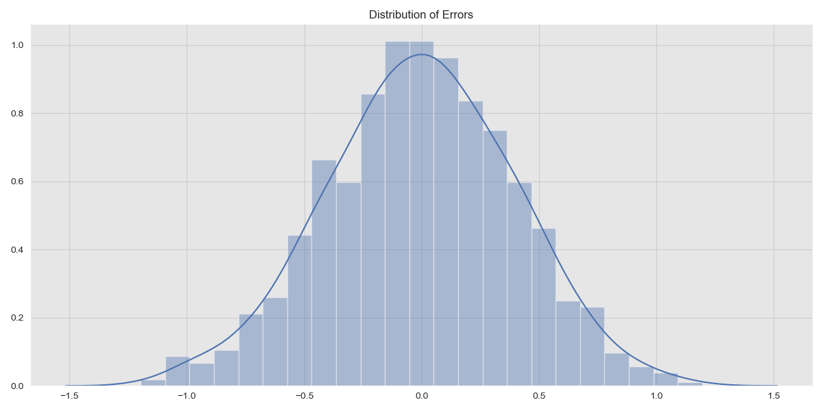Error Distribution

Kernel Functions

A Gaussian Process is entirely defined by its’ mean and kernel functions. For this post, we look only at the kernel function. In the case of Bayesian Linear Regression, a linear kernel is applied, allowing the model to find linear relationships between the covariates and outcomes. The Kernel Cookbook by David Duvenaud provides an excellent explanation of the different types of Kernel Functions available and their implications. We implement the Squared Exponential Kernel and the Rational Quadratic Kernel.

1
2
3
4
5
6
7
8
    def kernel_squared_exponential(x, y, sigma_f=1, l=1):
        K = sigma_f * np.exp( -(np.linalg.norm(x-y)**2)/(2* l**2) )
        return K

    def kernel_rational_quadratic(x, y, sigma_f=1, l=1, alpha=1):
        """ As alpha -> infinity, we get the squared exponential kernel """
        K = sigma_f * np.power(( 1 + (np.linalg.norm(x-y)**2)/(2*alpha*l**2) ), -alpha)
        return K

The Path to Inference

Generally, we are not interested in functions drawn from the prior as aren’t conditioned on any data. What we are interested in, however, is how to obtain the distribution of the posterior and an important step in that process is to characterise the joint distribution of training and test points.

Where \(K\) is the Kernel function. We want to find the conditional distribution \(f_* \vert f\) and we proceed as outlined in Section 2.3 of Pattern Recognition and Machine Learning (Bishop, 2006) and obtain the parameters of the conditional distribution:

However, this assumes that training data contains non-noisy observations. In both the real world and in out generated dataste, we consider observations of the form \(y = f(x) + \epsilon\) with noise variance \(0.4^2\). Noise is iid, therefore the variance of \(x\), \(var(x) = cov(x, x) = K(x, x) + \sigma_n^2 I\). This leads to a change in the parameters of the conditional distribution \(f_* \vert f\):

We take the mean function to be zero, leading to \(\mu_f = \mu_{f_*} = 0\).

We now write a function to compute the covariance kernels.

1
2
3
4
5
6
7
8
9
10
11
12
13
14
15
    def get_covariance_matrices(x, x_star, sigma_f=1, l=1, kernel_function=kernel_squared_exponential):
        """
        K = K(x, x)
        K_s = K(x*, x)
        K_ss = K(x*, x*)
        """
        
        n = x.shape[0]
        n_s = x_star.shape[0]
        
        K = np.array([[kernel_function(i, j, sigma_f=sigma_f, l=l) for i in x] for j in x])
        K_s = np.array([[kernel_function(i, j, sigma_f=sigma_f, l=l) for i in x_star] for j in x])
        K_ss = np.array([[kernel_function(i, j, sigma_f=sigma_f, l=l) for i in x_star] for j in x_star])
        
        return K, K_s, K_ss

Generating Test Points and Visualising

We generate 100 test points and select the parameters for the Squared Exponential kernel, choosing \(l = 0.1, \sigma_f = 1\). We then proceed to compute the covariance matrices for the training and test data.

1
2
3
4
5
6
7
8
9
10
11
12
13
14
    # Generate some test data points

    n_star = 100
    x_star = np.linspace(0, 1, n_star)

    f_x_star = f(x_star)

    # Choose kernel functions parameters
    sigma_f = 0.1
    l = 0.1
    #alpha = 1

    # Get the covariance matrices
    K, K_s, K_ss = get_covariance_matrices(x, x_star, sigma_f=sigma_f, l=l, kernel_function=kernel_squared_exponential)

We can visualise the covariance matrices, looking at the covariance between various observations.

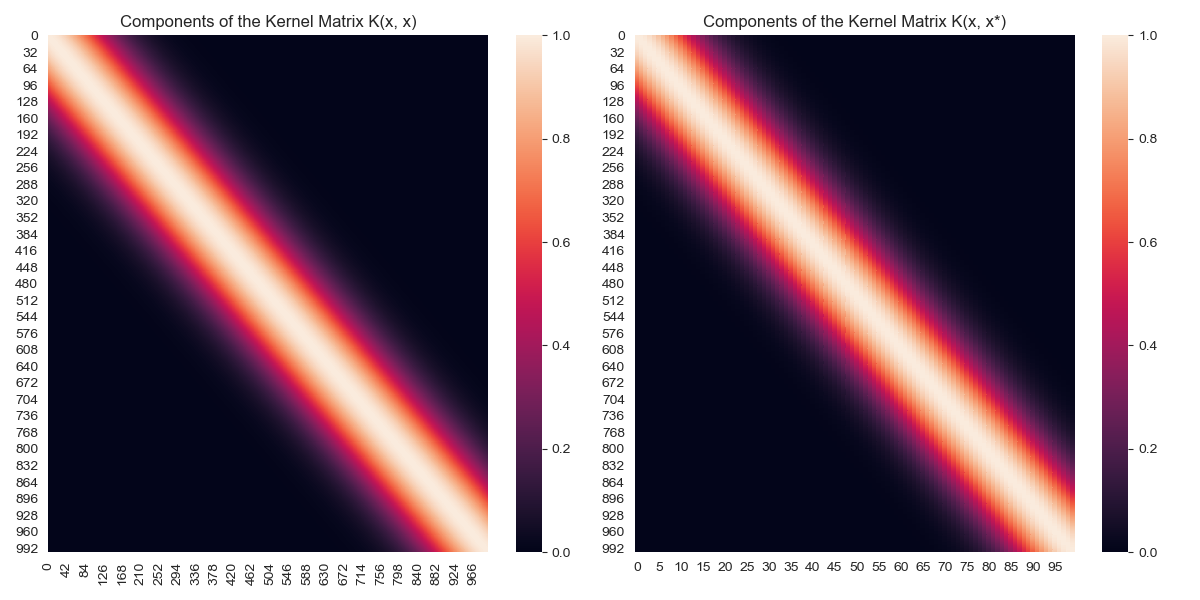Covariance heatmap for \(K(x,x), K(x,x_*)\)

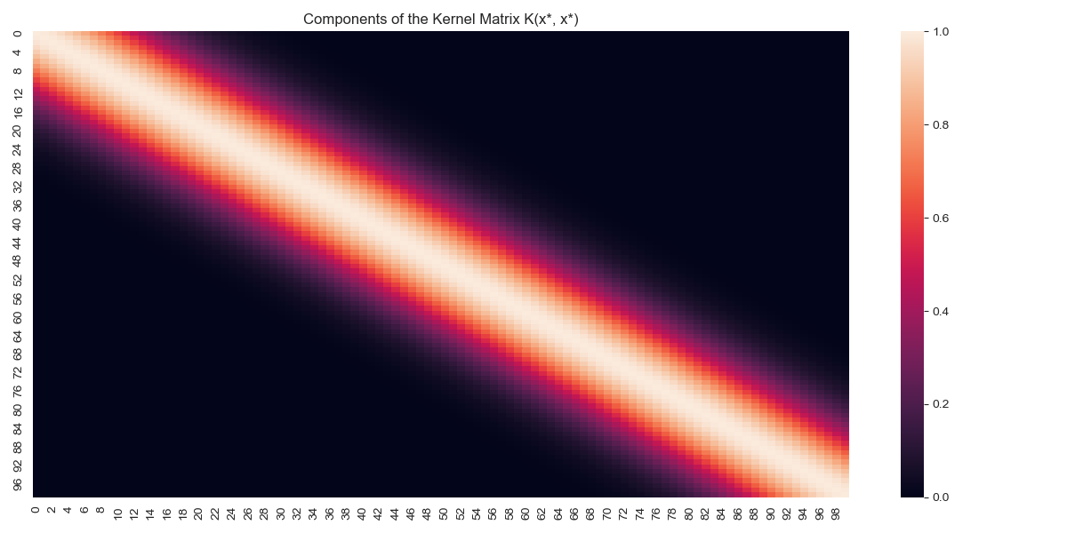Covariance heatmap for \(K(x_*,x_*)\)

Finally, although of little practical interest, we can draw samples from the prior and look at these. The prior has the distribution \(f_* \sim \mathcal{N}(0, K(x_*, x_*))\) and we can sample from it as follows:

1
2
3
4
5
6
7
8
9
10
11
12
    num_samples = 15
    fig, ax = plt.subplots()

    for _ in range(num_samples):
        sample = np.random.multivariate_normal(mean=np.zeros(n_star), cov=K_ss)
        sns.lineplot(x_star, sample, ax=ax, alpha=0.3, color="blue")

    # Plot f(x)
    sns.lineplot(x, f(x), color="red", ax=ax, label="f(x)")
    ax.set(title='Samples from Prior Distribution')
    plt.tight_layout()
    plt.show()

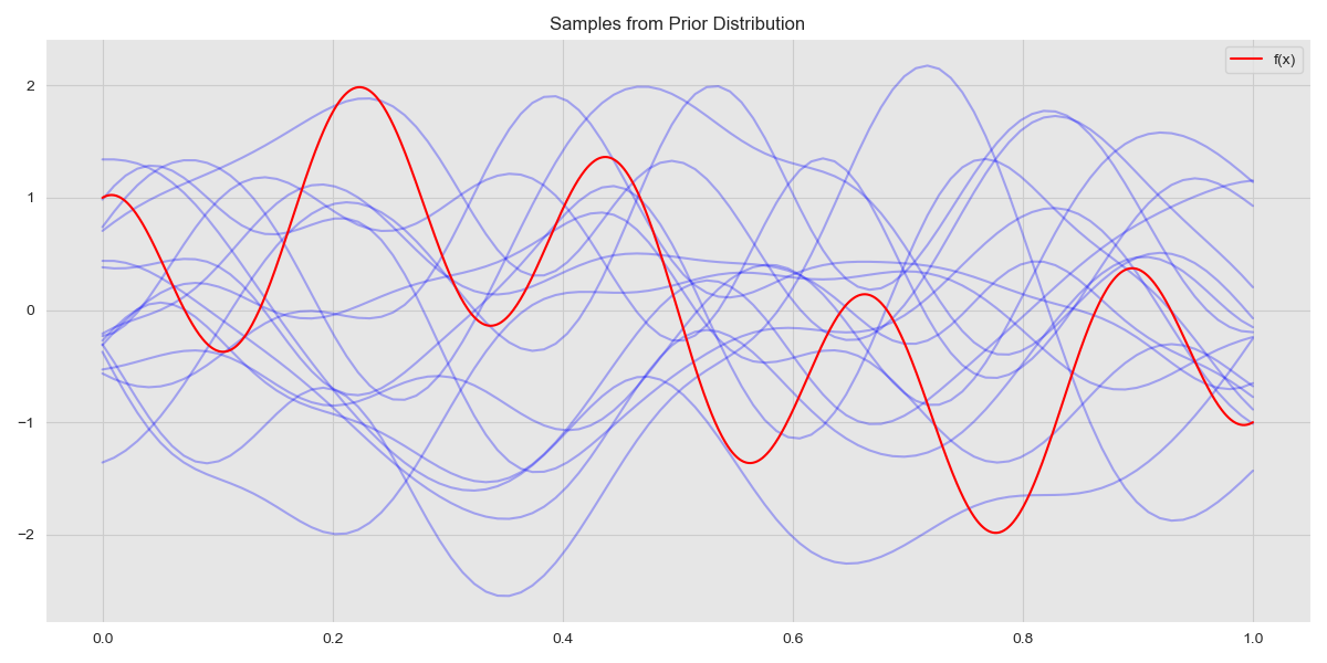Samples from Prior

Computing the Posterior

With the core machinery in place, we can now compute the parameters of the posterior distribution. We compute both \(\mu_{f_* \vert f}\) and \(\Sigma_{f_* \vert f}\) as

1
2
    f_star_mean = np.dot(K_s.T, np.dot(np.linalg.inv(K + np.eye(n)*sigma_n**2), y))
    f_star_cov = K_ss - np.dot(np.dot(K_s.T, np.linalg.inv(K + np.eye(n)*sigma_n**2)), K_s)

We draw samples from this distribution and plot.

1
2
3
4
5
6
7
8
9
10
11
12
13
    fig, ax = plt.subplots()
    num_samples = 100

    for _ in range(num_samples):
        # Sample from posterior distribution. 
        sample = np.random.multivariate_normal(mean=f_star_mean.reshape(-1), cov=f_star_cov)
        sns.lineplot(x=x_star, y=sample, color="blue", alpha=0.3, ax=ax);
        
    sns.lineplot(x, f(x), color='red', label = 'f(x)', ax=ax)
    sns.scatterplot(x, y, color='green', label = 'training points', ax=ax)
    ax.set(title=f'Samples of Posterior, sigma_f = {sigma_f} and l = {l}')
    plt.tight_layout()
    plt.show()

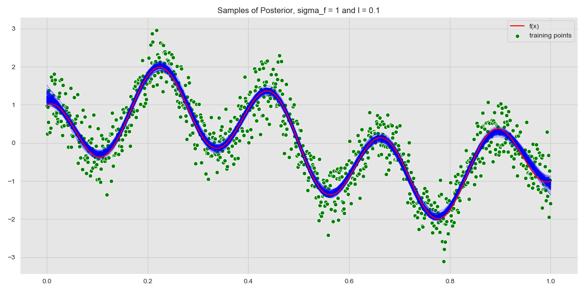Samples from Posterior

We can also look at the uncertainty of the model by plotting the regions within \(n\) standard deviations. We plot the posterior with the 2 standard deviation boundary, which is the 95% confidence interval.

1
2
3
4
5
6
7
8
9
    fig, ax = plt.subplots()
    std = np.sqrt(f_star_cov.diagonal())
    ax.fill_between(x_star, f_star_mean-2*std, f_star_mean+2*std, color="blue", alpha=0.3, label="2 SD");
    sns.lineplot(x, f(x), color='red', label = 'f(x)', ax=ax)
    sns.lineplot(x_star, f_star_mean, color='blue', label = 'Posterior mean', ax=ax)
    sns.scatterplot(x, y, color='green', label = 'training points', ax=ax)
    ax.set(title=f'Samples of Posterior, sigma_f = {sigma_f} and l = {l}')
    plt.tight_layout()
    plt.show()

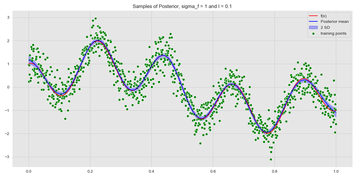Posterior with Confidence Interval

Straying Further Out

Next, we look into how the Gaussian Process behaves when performing inference on data it has never seen before – this has particular applications in time-series modelling. The paper Gaussian Processes for Timeseries Modelling tackles this in detail and is recommended reading for more information when dealing with time-series.

We look at how the model behaves, paying particular attention to the model uncertainty when we perform inference on data that is not in the region of the training set. Note that only the test data changes here, with training data in the region \([0, 2]\).

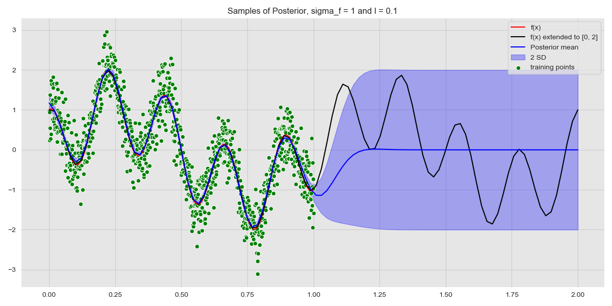Predicting on Out of Sample Data

As expected, we see near-identical performance in the region \([0, 1]\). What is more interesting, however, are the uncertainty bounds – as soon as we stray from the region covered by the training data, the model uncertainty blows up! This serves to highlight the power of Gaussian Processes, because, when a GP isn’t sure it reflects this in the uncertainty.

There is so much more to Gaussian Processes. We can achieve so much more by merely making better choices of Kernel (or Kernel combinations) as well as choosing hyperparameters for each kernel. We can also extend Gaussian Processes to classification problems. Recommended reading for all this and more is the GPML book.