We have all heard of Warren Buffet. The Oracle of Omaha, as of 2019, has achieved an average annual return of 20.5%. This far beats the average inflation rate of 9.95% per year since 1965. Compound interest means that $1 invested in 1965 is now worth over $23,000!
This begs the question: how do we get in on that sweet, sweet return? This is what quantitative aims to do. In quantitative finance, we analyse large datasets to best predict how well an asset will perform in the future. Most obviously, this data includes past information on stick prices. Many interesting strategies often make use of other data, such as news and tweets to perform sentiment analysis and attempt to understand how people perceive a stock. In this post we limit ourselves to past price data only and aim to gain an initial understanding of the task at hand.
Obtaining Data
All data science project rely on one thing – acquisition of good data. Thankfully, historical ticker data is easily obtained from Yahoo! Finance via the pandas-datareader package. A few lines of code later we can obtain historical data for any publicly traded stock.
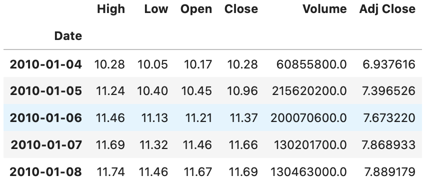 Ford Historical Prices
We focus on the Adj Close price, which stands for Adjusted Close as this is the closing price per share after adjusting for a corporate action such as a stock split.
Moving Average Trading
We first look into a very simple model of trading that, intuitively, says buy when we think the stock price is going to increase and sell when we think it is going to decrease.
This is achieved by finding a crossover point – a point at which we have an indication that a significant change in price is likely to occur. We make use of a \(N\) day Moving Average where each term is weighted equally, defined as:
\[\begin{align} MA=\frac{1}{N}\sum_{n=1}^{n=N} x_n \end{align}\]We also consider an Exponential Moving Average more recent terms are weighted more than older ones:
\[\begin{align} EMA= x_N + (1-\alpha) x_{N-1} + (1-\alpha)^2 x_{N-2} + ... + (1-\alpha)^N x_0 \end{align}\]where \(\alpha\) is a discounting term. A higher \(\alpha\) means older terms carry less weight and so the average relies more on recent values.
A moving average can be calculated for \(N\) past periods. Plotted below are the moving averages for Ford Adjusted Close prices, plotted alongside the true price.
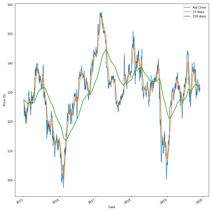 Ford Moving Average Prices Visualisation
When computing the moving average over a large window of time, 150 days, we see that the moving average does not closely mirror the true price at all – it is too smoothed. Thus it is important to choose an appropriate window length when using the moving average.
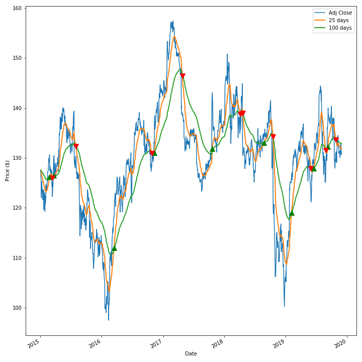
We now introduce the Moving Average (MA) trading strategy. With the MA strategy we compute two moving averages for the same stock, each of different lengths. When the short window MA price drops below the long window MA, we sell shares in the stock and vice versa when the short window MA rises above the long window MA. We implement this strategy with both a simple MA as well as an exponential MA and compare both against a more Buffet-ian strategy of buying and holding.
Without further ado, let’s see how well this strategy performs. Initially, choosing a short window of 25 days and a long window of 100 days we attempt this strategy using both types of MA for the stock IBM, between 2015 and December 2019 (to avoid COVID-19 effects).
 IBM MA Strategy
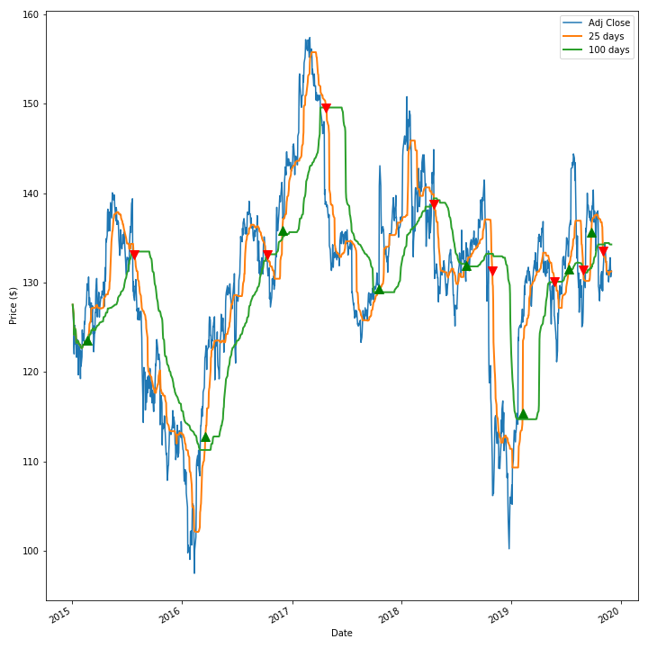
 IBM Exponential MA Strategy
In the spirit of exploration, we also consider a different version of the MA trading strategy, a moving Median Average (MdA) where rather than computing the mean of a set of terms, we instead use the median value. Why a median? As a median is the central value in a sorted sequence, then it is more robust against outliers and as a result, smoothing with a moving median should yield a curve with fewer sharp spikes.
 IBM MdA Strategy
The next question is, just how successful are these strategies? We summarise our strategies’ performance over the 4.92 years used for backtesting, below:
| Strategy | % Improvement over Buy and Hold | Absolute Return ($) | Number of Trades |
|---|---|---|---|
| Moving Average | -762.54 | -24.97 | 16 |
| Moving Median | -578.17 | -18.02 | 16 |
| Exponential Moving Average | -1019.94 | -34.67 | 20 |
| Buy and Hold | NA | 3.77 | 1 |
The results paint a grim picture. A Moving Median/Average strategy underperforms compared to a buy and hold strategy and suggests that a strategy that involves buying when a stock looks like it is about to move up and selling before it looks to be moving down significantly isn’t profitable. Clearly more there is more to making money from the stock market.